Internet provides access to plethora of information today. Whatever we need is just a Google (search) away. However, when we have so much of information, the challenge is to segregate between relevant and irrelevant information.
When our brain is fed with a lot of information simultaneously, it tries hard to understand and classify the information between useful and not-so-useful information. We need a similar mechanism to classify incoming information as useful or less-useful in case of Neural Networks.
This is a very important in the way a network learns because not all information is equally useful. Some of it is just noise. Well, activation functions help the network do this segregation. They help the network use the useful information and suppress the irrelevant data points.
Let us go through these activation functions, how they work and figure out which activation functions fits well into what kind of problem statement.
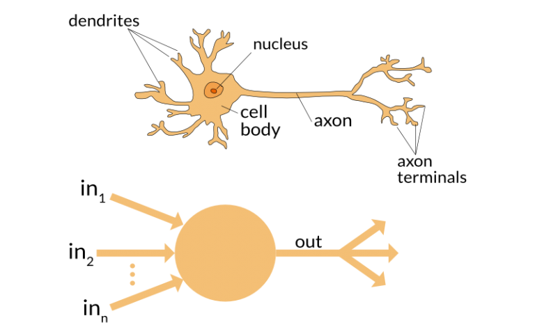
Before I delve into the details of activation functions, let’s do a little review of what are neural networks and how they function. A neural network is a very powerful machine learning mechanism which basically mimics how a human brain learns. The brain receives the stimulus from the outside world, does the processing on the input, and then generates the output.
As the task gets complicated multiple neurons form a complex network, passing information among themselves.
Using a artificial neural network, we try to mimic a similar behavior. The network you see below is a neural network made of interconnected neurons.
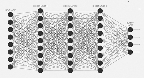
The black circles in the picture above are neurons. Each neuron is characterized by its weight, bias and activation function. The input is fed to the input layer. The neurons do a linear transformation on the input by the weights and biases. The non linear transformation is done by the activation function. The information moves from the input layer to the hidden layers. The hidden layers would do the processing and send the final output to the output layer. This is the forward movement of information known as the forward propagation. But what if the output generated is far away from the expected value? In a neural network, we would update the weights and biases of the neurons on the basis of the error. This process is known as back-propagation. Once the entire data has gone through this process, the final weights and biases are used for predictions.
Activation functions are an extremely important feature of the artificial neural networks. They basically decide whether a neuron should be activated or not. Whether the information that the neuron is receiving is relevant for the given information or should it be ignored.
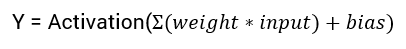
The activation function is the non linear transformation that we do over the input signal. This transformed output is then sen to the next layer of neurons as input.
Now the question which arises is that if the activation function increases the complexity so much, can we do without an activation function?
When we do not have the activation function the weights and bias would simply do a linear transformation. A linear equation is simple to solve but is limited in its capacity to solve complex problems. A neural network without an activation function is essentially just a linear regression model. The activation function does the non-linear transformation to the input making it capable to learn and perform more complex tasks. We would want our neural networks to work on complicated tasks like language translations and image classifications. Linear transformations would never be able to perform such tasks.
Activation functions make the back-propagation possible since the gradients are supplied along with the error to update the weights and biases. Without the differentiable non linear function, this would not be possible.
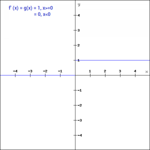
The first thing that comes to our mind when we have an activation function would be a threshold based classifier i.e. whether or not the neuron should be activated. If the value Y is above a given threshold value then activate the neuron else leave it deactivated.
It is defined as –
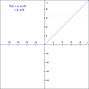
f(x) = 1, x>=0
= 0, x<0
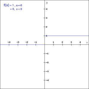
The binary function is extremely simple. It can be used while creating a binary classifier. When we simply need to say yes or no for a single class, step function would be the best choice, as it would either activate the neuron or leave it to zero.
The function is more theoretical than practical since in most cases we would be classifying the data into multiple classes than just a single class. The step function would not be able to do that.
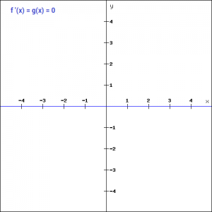
Moreover, the gradient of the step function is zero. This makes the step function not so useful since during back-propagation when the gradients of the activation functions are sent for error calculations to improve and optimize the results. The gradient of the step function reduces it all to zero and improvement of the models doesn’t really happen.
f '(x) = 0, for all x
We saw the problem with the step function, the gradient being zero, it was impossible to update gradient during the backpropagation. Instead of a simple step function, we can try using a linear function. We can define the function as-
f(x)=ax
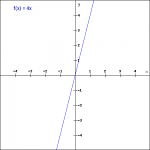
We have taken a as 4 in the figure above. Here the activation is proportional to the input. The input x, will be transformed to ax. This can be applied to various neurons and multiple neurons can be activated at the same time. Now, when we have multiple classes, we can choose the one which has the maximum value. But we still have an issue here. Let’s look at the derivative of this function.
f'(x) = a
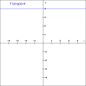
The derivative of a linear function is constant i.e. it does not depend upon the input value x.
This means that every time we do a back propagation, the gradient would be the same. And this is a big problem, we are not really improving the error since the gradient is pretty much the same. And not just that suppose we are trying to perform a complicated task for which we need multiple layers in our network. Now if each layer has a linear transformation, no matter how many layers we have the final output is nothing but a linear transformation of the input. Hence, linear function might be ideal for simple tasks where interpretability is highly desired.
Sigmoid is a widely used activation function. It is of the form-
f(x)=1/(1+e^-x)
Let’s plot this function and take a look of it.
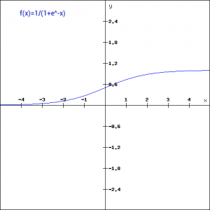
This is a smooth function and is continuously differentiable. The biggest advantage that it has over step and linear function is that it is non-linear. This is an incredibly cool feature of the sigmoid function. This essentially means that when I have multiple neurons having sigmoid function as their activation function – the output is non linear as well. The function ranges from 0-1 having an S shape. Let’s take a look at the shape of the curve. The gradient is very high between the values of -3 and 3 but gets much flatter in other regions. How is this of any use?
This means that in this range small changes in x would also bring about large changes in the value of Y. So the function essentially tries to push the Y values towards the extremes. This is a very desirable quality when we’re trying to classify the values to a particular class.
Let’s take a look at the gradient of the sigmoid function as well.
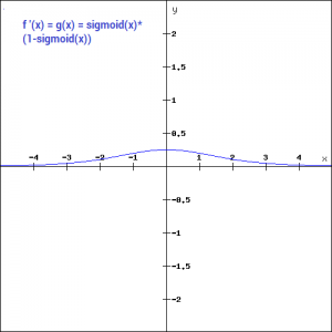
It’s smooth and is dependent on x. This means that during backpropagation we can easily use this function. The error can be backpropagated and the weights can be accordingly updated.
Sigmoids are widely used even today but we still have a problems that we need to address. As we saw previously – the function is pretty flat beyond the +3 and -3 region. This means that once the function falls in that region the gradients become very small. This means that the gradient is approaching to zero and the network is not really learning.
Another problem that the sigmoid function suffers is that the values only range from 0 to 1. This meas that the sigmoid function is not symmetric around the origin and the values received are all positive. So not all times would we desire the values going to the next neuron to be all of the same sign. This can be addressed by scaling the sigmoid function. That’s exactly what happens in the tanh function. let’s read on.
The tanh function is very similar to the sigmoid function. It is actually just a scaled version of the sigmoid function.
tanh(x)=2sigmoid(2x)-1
It can be directly written as –
tanh(x)=2/(1+e^(-2x)) -1
Tanh works similar to the sigmoid function but is symmetric over the origin. it ranges from -1 to 1.
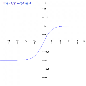
It basically solves our problem of the values all being of the same sign. All other properties are the same as that of the sigmoid function. It is continuous and differentiable at all points. The function as you can see is non linear so we can easily backpropagate the errors.
Let’s have a look at the gradient of the tan h function.
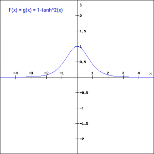
The gradient of the tanh function is steeper as compared to the sigmoid function. Our choice of using sigmoid or tanh would basically depend on the requirement of gradient in the problem statement. But similar to the sigmoid function we still have the vanishing gradient problem. The graph of the tanh function is flat and the gradients are very low.
The ReLU function is the Rectified linear unit. It is the most widely used activation function. It is defined as-
f(x)=max(0,x)
It can be graphically represented as-
ReLU is the most widely used activation function while designing networks today. First things first, the ReLU function is non linear, which means we can easily backpropagate the errors and have multiple layers of neurons being activated by the ReLU function.
The main advantage of using the ReLU function over other activation functions is that it does not activate all the neurons at the same time. What does this mean ? If you look at the ReLU function if the input is negative it will convert it to zero and the neuron does not get activated. This means that at a time only a few neurons are activated making the network sparse making it efficient and easy for computation.
Let’s look at the gradient of the ReLU function.
But ReLU also falls a prey to the gradients moving towards zero. If you look at the negative side of the graph, the gradient is zero, which means for activations in that region, the gradient is zero and the weights are not updated during back propagation. This can create dead neurons which never get activated. When we have a problem, we can always engineer a solution.
Leaky ReLU function is nothing but an improved version of the ReLU function. As we saw that for the ReLU function, the gradient is 0 for x<0, which made the neurons die for activations in that region. Leaky ReLU is defined to address this problem. Instead of defining the Relu function as 0 for x less than 0, we define it as a small linear component of x. It can be defined as-
f(x)= ax, x<0
= x, x>=0
What we have done here is that we have simply replaced the horizontal line with a non-zero, non-horizontal line. Here a is a small value like 0.01 or so. It can be represented on the graph as-
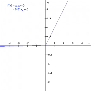
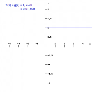
The main advantage of replacing the horizontal line is to remove the zero gradient. So in this case the gradient of the left side of the graph is non zero and so we would no longer encounter dead neurons in that region. The gradient of the graph would look like –
Similar to the Leaky ReLU function, we also have the Parameterised ReLU function. It is defined similar to the Leaky ReLU as –
f(x)= ax, x<0
= x, x>=0
However, in case of a parameterised ReLU function, ‘a‘ is also a trainable parameter. The network also learns the value of ‘a‘ for faster and more optimum convergence. The parametrised ReLU function is used when the leaky ReLU function still fails to solve the problem of dead neurons and the relevant information is not successfully passed to the next layer.
The softmax function is also a type of sigmoid function but is handy when we are trying to handle classification problems. The sigmoid function as we saw earlier was able to handle just two classes. What shall we do when we are trying to handle multiple classes. Just classifying yes or no for a single class would not help then. The softmax function would squeeze the outputs for each class between 0 and 1 and would also divide by the sum of the outputs. This essentially gives the probability of the input being in a particular class. It can be defined as –
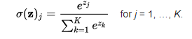
Let’s say for example we have the outputs as-
[1.2 , 0.9 , 0.75], When we apply the softmax function we would get [0.42 , 0.31, 0.27]. So now we can use these as probabilities for the value to be in each class.The softmax function is ideally used in the output layer of the classifier where we are actually trying to attain the probabilities to define the class of each input.
Now that we have seen so many activation functions, we need some logic / heuristics to know which activation function should be used in which situation. Good or bad – there is no rule of thumb.
However depending upon the properties of the problem we might be able to make a better choice for easy and quicker convergence of the network.
In this article I have discussed the various types of activation functions and what are the types of problems one might encounter while using each of them.
I would suggest to begin with a ReLU function and explore other functions as you move further. You can also design your own activation functions giving a non-linearity component to your network. If you have used your own activation function which worked really well, please share it with us and we shall be happy to incorporate it into the list.